

Introduction
The Arm Cortex-M55 is the first released CPU based on the Armv8.1-M architecture – the biggest architectural revision so far to the M-profile, in terms of its effect on general application code. As such it is very much the cutting edge of Arm microcontrollers, and this is reflected in the maturity of library and tooling technology. As of late 2022, very few silicon implementations are on the market, and most of the software support was created during 2019–2021 but has yet to be shaken out in deployment.
This whitepaper looks at the comparative performance of current toolchains for the Cortex-M55 CPU as used in Alif MCUs and Fusion Processors and digs into the background, and the underlying new optimization issues.
Scope of this study
This study only looked at code for the RTSS subsystem – running on a Cortex-M55 in either the RTSS-HE or RTSS-HP part of the device. There is a brief supplement note about the Cortex-A32. Compilers used were Arm Compiler 6.18 and GCC 11.3 packaged as Arm GNU Toolchain 11.3.Rel1 – the latest “release” versions as of October 2022.
Compiler versions from 2021 or earlier will have limited or buggy Cortex-M55 support and are not recommended.
Arm Compiler 6 is available commercially as either as part of Arm’s Development Studio (Linux or Windows), or Keil MDK (Windows only), and there is no difference in code generation capability between the packages.
GCC is available free as part of Arm GNU Toolchain.
Compilation example 1 – image manipulation
The first compiler comparison comes from some simple code used as part of an image classification machine-learning (ML) demo, to process camera data before feeding it to the ML model.
There are five stages:
- Convert a captured 560×560 Bayer-tiled image to conventional 560×560 24-bit RGB.
- Crop the image (degenerate case to 560×560, so effectively a memcpy).
- Bilinear interpolate to 224×224.
- Apply a colour-correction matrix.
- Paint the 224×224 image to the LCD framebuffer, pixel doubled.
This is the sort of CPU-intensive activity that has quite a lot of scope for micro-optimisation and is particularly amenable to application of the Helium vector unit. (Although some of the operations could more effectively be performed using the dedicated GPU2D hardware unit.)
The original code was very generic C, with no particular effort made to speed optimize or special case.
Code was executed on the High-Performance core.
Using various optimization levels, the resulting read-only code size is shown in Figure 1. The large image classification neural net model (3.5MiB) was excluded from the total, to make the comparison more representative of general code. There will still be other read-only data tables of fixed size, meaning the actual code size difference will be a little greater than indicated.

Both compilers produce much bigger code at -O0, and this can cause problems fitting into the device. The compilers respectively advise use of -O1 (clang) or -Og (gcc) for usual debugging, and this produces size more comparable to release builds.
armclang produced 8–15% smaller code at each optimization level. GCC 11 does not have the size-minimising level -Oz, but this is coming in later versions. armclang’s -Oz was 17% smaller than GCC’s -Os.
GCC suffers a particular code size increase at -O3 – this is the level at which it activates auto-vectorization, and it is due to not taking full advantage of Helium’s tail predication feature (see below). armclang’s -O2 is 16% smaller than GCC’s -O3, and is still 13% faster. Unlike gcc, vectorisation in armclang is activated at -O2.
Figure 2 shows total execution time for the 5 steps. As expected, -O0 has a serious impact, while above -O1/-Og, execution time decreases as you would expect, being a mirror image of the size increase.

armclang’s code took 16–30% less execution time than gcc’s at the same level, equivalent to a 20–44% speedup. armclang’s -Oz took 10% less time than GCC’s -Os, while still being 17% smaller.
Figure 3 shows the five stages of the algorithm in more detail for full optimisation levels, and we can start to break down the optimisation possibilities.
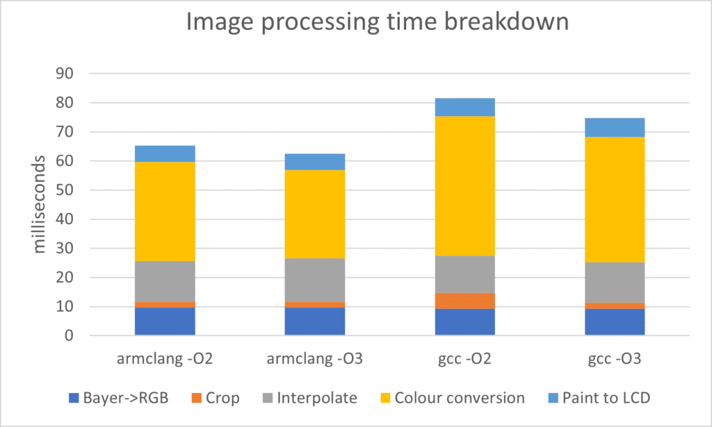
Although all stages have some scope for auto-vectorisation, in the original code, only the crop stage was auto-vectorised. The lack of vectorisation in gcc -O2 is clearly visible.
The first and easiest optimisation was to the longest-running stage. All that was required was to eliminate the use of double-precision floating point in the matrix conversion:
float32_t spixel_data[3];
uint8_t *sp;
dpixel_data[0] = 2.092*sp[2] – 0.369*sp[1] – 0.636*sp[0];
dpixel_data[1] = -0.492*sp[2] + 1.315*sp[1] + 0.162*sp[0];
dpixel_data[2] = -0.139*sp[2] – 0.664*sp[1] + 3.017*sp[0];
Although the intent was presumably to use single-precision, the lack of an f suffix on the constants forced the expression to be computed in double-precision. Adding f to make the constants be of type float reduces the execution time from 30ms to under 5ms ((armclang -O3).
Although the Cortex-M55 does have hardware double-precision support, it is an area-optimized implementation, and is much slower than its single-precision or half-precision. There is also no ability to vectorize double operations, so use of double should still be avoided.
Other simple optimisations were possible by the pixel doubling operate word-at-a-time rather than byte-at-a-time, and making the generic code non-generic by adding
if (bpp != 24) abort();
This was a simple patch in a couple of functions which allowed the compiler to know the value of bpp below those tests (thanks to abort being a noreturn function) and reduce the generic code to optimised 24-bpp code, without any further code restructuring.
These changes and addition of some restrict keywords enabled some more auto-vectorisation, including the pixel doubling. See below for more notes on restrict.
Final optimisation came from using Helium intrinsics to manually vectorize the various stages, either by processing the three color channels from one pixel in parallel (relatively easy) or by processing one color channel from 8 or 16 pixels in parallel (slightly trickier). The hand-tuned vector paint was only very slightly faster than the compiler’s version, but it was possible to vectorize the Bayer->RGB, interpolation and color correction that the compilers did not auto-vectorize.
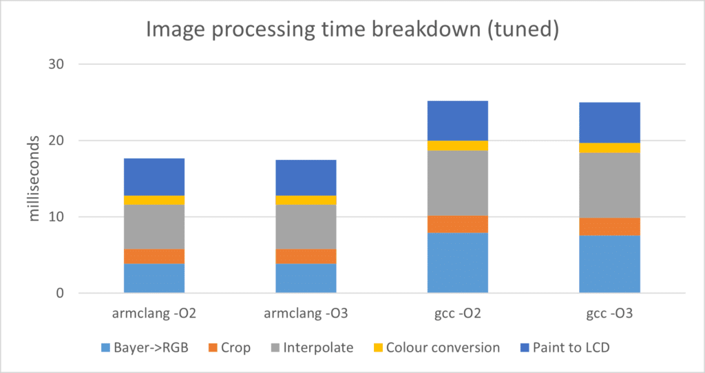
Figure 4 shows the final optimisation results. Despite the bulk of the code being now hand-tuned, and nearly four times faster, armclang still has the lead, with 30% less time spent, or a 42% speed increase. One confounding factor is that the Helium optimisation for the Bayer->RGB code did not compile on GCC due to a compiler bug (see Future toolchain development), and there was no straightforward workaround, so it is still using a pure C version. During development 3 or 4 bugs were found in GCC’s Helium intrinsic handling – most were worked around or ended up not being hit in the final version of the code.
Some fixes are queued up for GCC 13, others have yet to be resolved, including at least one -O3 failure in the absence of intrinsics.
Aside from that, GCC tends to more often insert extra unnecessary operations around intrinsics (or assembler), while armclang can create better Helium vector loops.
Compilation example 2 – keyword spotting
The second example is also from a machine learning demo. In this case we are looking at the complete pre-processing and inference time for an audio sample.
The demo in question is using TensorFlow Lite running on the Cortex-M55 in the High-Efficiency subsystem, with a model accelerated by the Ethos-U55 NPU.
Code size is shown in Figure 5. -O3 increases code size on both compilers, due to extra unrolling, and -Ofast adds extra optimisation on top of -O3 by permitting some deviations from the C standard, particularly in floating point computations, so it slightly reduces code size again. Armclang was 28–30% smaller in each case.
It’s likely that some of this significant difference could be due to differences in how much C library code was pulled in. This was not investigated.

The extra space taken by -O3 achieves little, as we can see in Figure 6. GCC was imperceptibly faster, and armclang was actually imperceptibly slower. Unrolling tends to be ineffective on the Cortex-M55, as discussed below.
The extra leniency granted by -Ofast does provide a notable boost though. It’s likely that -O2 together with the manual conformance relaxation options equivalent to -Ofast (-ffast-math, -ffp-mode=fast, etc) might be the best overall optimization choice in this case, although this combination was not tested. At -Ofast, armclang took 26% less time, or was 30% faster. With the keyword spotting being performed on 500ms intervals, this is the difference between 3% and 4% CPU utilization, with a corresponding difference in power consumption.

This keyword spotting example has a relatively simple inference stage in the model, but a large amount of floating-point DSP work is required to compute the Mel-Frequency Cepstral Coefficients (MFCCs) that the model accepts as inputs. Of the total runtime, a fixed 3.35ms is taken by the inference running on the Ethos-U55, and this does not vary depending on the compiler or its options, but the bulk of the time is taken up by the DSP pre-processing work on the Cortex-M55, and this is very compiler-dependent, ranging from 14.6 to 21.9ms.
This DSP work is mostly performed by Helium-optimised vector code using FFT and other routines from CMSIS-DSP. A few concluding steps for each MFCC are performed using scalar square root and logarithm operations, but they are a small proportion. The results demonstrates that even heavily Helium-intrinsic-optimized code is still very dependent on the toolchain for performance. Only direct assembler optimization would be toolchain independent.
(Note that one fairly straightforward optimisation was not being performed in this test code – as it’s examining overlapping 1-second samples, half the MFCCs can be reused from the previous window, halving the DSP time. This optimisation had been omitted to simplify some automatic gain handling).
Cortex-M55 (ARMv8.1-M with MVE) code generation
Having looked at the results, we can look a bit deeper at the code generation issues new to the Cortex-M55, with its new architecture. Arm Compiler has historically always had something of an edge over GCC, but the gap is particularly large at present for the M55, and we can investigate why.
Helium (aka the M-Profile Vector Extension [MVE])
The M-Profile Vector Extension (MVE) is a new vector instruction set that permits operation on 128-bit vectors, viewed as 8-, 16- or 32-bit signed or unsigned integers, 16- or 32-bit floating point numbers, or as 128-bit units for big-number cryptographic operations. The vectors re-use the 32-single/16-double floating-point register file, reinterpreting it as eight quad-word registers Q0 to Q7.
This is similar in concept to Neon (Advanced SIMD) from the A-Profile, but is adapted to work without requiring a full 128-bit data path, and it backports various concepts from Arm’s Scalar Vector Extension, making it simpler to use than Neon, and adds refinements such as being able to take scalar values from general-purpose registers, meaning that there is less demand for the reduced number of vector registers.
Cortex-M55’s MVE implementation uses a 64-bit data path, so it processes 2 32-bit “beats” per cycle, leading to 2 cycles per instruction. Data processing can be interleaved with loads or stores for a 1 cycle per operation throughput. (The MVE instruction set architecture is designed to permit 1 or 4 beats per cycle for lower or higher performance implementations, although no instances yet exist).
Simple example:
VLDRB.S8 Q0,[R0],#16 ; load 16 bytes into Q0 and advance the pointer
VLDRB.S8 Q1,[R1],#16 ; load 16 bytes into Q1 and advance the pointer
VHADD.S8 Q0,Q0,Q1 ; halve and add the 16 bytes
; Q0[n] := (Q0[n] + Q1[n]) / 2 VSTRB.S8 Q0,[R2],#16 ; store 16 results and advance the pointer
This would take 7 cycles for the loads and stores and 16 additions; the second VLDRB and the VHADD would overlap.
These sorts of vector instructions do not naturally align with normal high-level language constructs, so generating them requires sophisticated compiler auto-vectorisation that can detect patterns that can be safely turned into vectors, or manual coding using special intrinsics or assembly.
Both GCC and armclang are capable of auto-vectorisation – armclang enables it at optimization level -O2 or higher, and GCC enables it at -O3.
Auto-vectorization is fragile – the compiler must be able to prove that accesses do not overlap. This is very hard in C/C++ when using pointers, unless the restrict keyword is used. Data in separate arrays permits the optimisation more often.
// This could be vectorised, as the compiler could deduce that
// the output does not affect the input.
void average1(uint8_t *data, size_t n)
{
for (size_t i = 0; i < n; i++)
data[i] = (data[i * 2] + data[i * 2 + 1]) / 2;
}
// This cannot generally be vectorised, as the compiler can’t tell
// whether in and out overlap, so it is compelled to work one
// element at a time to get all possible overlap cases right.
void average2(uint8_t *out, const uint8_t *in, size_t n)
{
for (size_t i = 0; i < n; i++)
out[i] = (in[i * 2] + in[i * 2 + 1]) / 2;
}
// This can be vectorised, as restrict tells the compiler
// that in and out cannot overlap
void average3(uint8_t * restrict out, const uint8_t * restrict in, size_t n)
{
for (size_t i = 0; i < n; i++)
out[i] = (in[i * 2] + in[i * 2 + 1]) / 2;
}
extern uint8_t in_array[], out_array[];
// This can be vectorised, as the compiler can see that
// we’re accessing two different arrays.
void average4(size_t n)
{
for (size_t i = 0; i < n; i++)
out_array[i] = (in_array[i * 2] + in_array[i * 2 + 1]) / 2;
}
There are further restrictions with vectorising floating-point code, as the vector form may not fully preserve IEEE-754 exception semantics, so compiler options or pragmas to relax conformance may be required, as per the discussion of -Ofast above.
Even if auto-vectorization is possible, the main penalty has traditionally been that unless the compiler can deduce that a loop is a multiple of the vector size, it must also incorporate scalar tail handling to handle the remainder, so vectorized code is usually significantly bigger. However, this is not necessarily the case with Helium. We will return to this.
Low-overhead branches
M-Profile Arm processors do not have the sort of branch predictor seen on A-Profile devices or other full-powered CPUs, due to the energy and die space overhead. Armv8.1-M introduces an architectural extension that allows counted loops to have effectively zero overhead, without a general prediction unit. By using the “Loop Start” and “Loop End” instructions the the processor can predict the branch back to the start of the innermost loop.
Consider a simple example using ARMv7-M (or ARMv8.0-M) code:
; void *memset_v7(void *dst, int ch, size_t count)
memset_v7:
PUSH {R0, LR}
CBZ R2, end ; branch to end if 0
loop: STRB R1, [R0], #1 ; store ch to r0, advancing pointer (1 or 2 cycles)
SUBS R2, R2, #1 ; decrement loop counter (1 cycle)
BNE loop ; branch back if non-zero (2 or 3 cycles)
end: POP {R0, PC}
This naïve code is not very efficient, as less than half the execution time is spent doing stores – the rest is spent decrementing the counter and branching, so there is a huge gain to be had from unrolling. But the situation for ARMv8.1-M is very different:
; void *memset(void *dst, int ch, size_t count)
memset:
PUSH {R0, LR}
WLS LR, R2, end ; start while loop count r1, branch to end if 0
loop: STRB R1, [R0], #1 ; store ch to r0, advancing pointer
LE LR, loop ; decrement loop counter, branch back if non-zero
end: POP {R0, PC}
This will execute with no branch overhead, as the LE instruction will not actually be executed after the first iteration. Rather, the processor will use cached loop information to execute back-to-back STRB instructions with no branch penalty. Also, note that the decrement of the loop counter is also free – it’s a dedicated CPU function like the program counter, rather than having to go via the main arithmetic unit. Effective instruction flow for 4 iterations would be:
PUSH {R0, LR}
WLS LR, R2, end ; LR := 4
STRB R1, [R0], #1
LE LR, loop ; LR := 3, fill loop info, branch
; (only) branch penalty
STRB R1, [R0], #1 ; LR := 2
STRB R1, [R0], #1 ; LR := 1
STRB R1, [R0], #1 ; LR not decremented to 0, but LE skipped
POP {R0, PC}
Thus there is generally no little or no benefit to simple loop unrolling. It could benefit from larger accesses, but not just unrolling.
This mechanism only works at one layer of loops, and ones which do not call subroutines, but these are often the most speed-critical and where there is the most to be gained by eliminating branch overhead.
Both GCC and armclang support the new loop instructions, and routinely use them where appropriate when targeting Cortex-M55. (Support was not present in versions prior to GCC 11, so it is important to upgrade from GCC 10 or earlier.) However it does not appear that either armclang or GCC have had their unrolling heuristics tuned to account for normal loops being low-overhead, as both still tend to unroll at high optimisation levels, to little effect, as seen in the charts above. Some experimentation with unroll options may be worthwhile, although auto-vectorisation may rely on unrolling being enabled in general (as a vector operation is usually created more than one C loop iteration).
Tail predication
One key feature taken from SVE is per-lane predication, using a 16-bit mask register, which permits a range of sophisticated processing with vectorized “if/then” conditions. This can be used to handle conditional operations, such as clipping:
MOVS R0, #224
VPT.U8 HI, Q0, R0 ; Vector Predicate Test – combines VCMP and predicate setup
; set predicate mask selecting lanes > 224
; and start a 1-instruction predicated block
VDUPT.U8 Q0, R0 ; duplicate 224 into lanes greater than 224,
; leaving others untouched
(Instructions in a VPT block are conventionally marked with a T modifier, but this is not encoded in the instruction; it’s the VPT instruction that causes the predication for 1 to 4 following instructions).
Much more common though is the use of this logic for tail predication, which masks out unwanted excess operations at the end of a loop – something required in almost any generic data processing code.
Tail predication can be done “manually” by using the VCTP (Construct Tail Predicate) instruction to load a predicate mask based on a count value. This could be used to perform the last iteration of a loop.
VCTP.8 R0 ; set 0-16 bits in predicate mask
; (all bits set for any value of R0 >= 16)
VPSTTT ; start a 3-instruction predicated block
VLDRBT.U8 Q0, [R1] ; load 0-16 bytes (others set to zero)
VSHRT.U8 Q0, Q0, #1 ; halve 0-16 bytes (others left as-is)
VSTRBT.8 Q0, [R1] ; stores 0-16 bytes (others not written)
The above would also work for every iteration, although there would be unnecessary overhead from the VCTP and VPST instructions for every iteration before the last.
But in fact, there is no need to do this manually, as the Loop Start and Loop End instructions can do it for you. Revisiting the memset above, it could be vectorized thus:
; void *memset(void *dst, int ch, size_t count)
memset:
PUSH {R0, LR}
WLSTP.8 LR, R2, end ; start tail-predicated while loop
VDUP.8 Q0, R1
loop: VSTRB.8 Q0, [R0], #16 ; store 1-16 zeros, advancing pointer by 16
LETP LR, loop ; decrement loop counter by 16 and branch
; with special handling for last iteration
end: POP {R0, PC}
Due to the “TP” on the loop instruction, a predication mask from the loop counter is automatically applied to all instructions inside the loop (and combined with any explicit predication inside it – it’s a parallel masking mechanism).
This means that it is straightforward to process loops of arbitrary size using the vector operations. Unlike Neon code, there is no need to have separate scalar code to process the odd data that is not a multiple of the vector size.
And as before, there is no need to unroll – the CPU will execute back-to-back VSTRB.8 instructions, maximizing throughput. This means that, in principle, vectorization can be “free” in terms of code size. There is no speed/size trade-off. A vector implementation can often be the same number of instructions as a scalar implementation, or maybe even fewer, given that there are many operations available in the vector instruction set that are not present in the scalar set.
Unfortunately, GCC is presently incapable of using the tail-predicated loop instructions; it always generates scalar tail code similar to Neon code, meaning its auto-vectorisation has a significant size overhead, as well as not being as fast as it could be.
When writing Helium C intrinsics for manual optimisation, tail predication must be expressed using the vctpq() intrinsic and predicated operations, and it is up to the compiler to optimize these away and transform into a tail predicated loop. Only armclang can do this – GCC will generate lots of explicit VCTP and VPST instructions.
Helium intrinsic example
Here’s some of the optimized color-correction code to give an idea of what manual Helium optimisation in C code looks like. (This does not incorporate tail handling, on the assumption that the image is a multiple of 16 pixels – this slightly simplifies it).
// Prepare { 0, 3, 6, … 21 } offset array indexing 8 RGB pixels
// vidup is Vector Increment and Duplicate, starting at 0 and incrementing by 1
// and we multiply the result by 3.
const uint16x8_t pixel_offsets = vmulq(vidupq_n_u16(0, 1), 3);
while (len > 0) {
// Fetching 2 iterations ahead seems optimal for RTSS-HP from SRAM0
// Cortex-M55 has automatic prefetch, but a manual prefetch hint still
// helps for this particular loop
__builtin_prefetch(sp + 3 * 8 * 2);
// Use gather loads to separate R,G,B for 8 pixels into 3 Q registers
// converting from uint8_t to float16_t. Note the extensive use of
// generic functions – type is only stated where it can’t be deduced
// from arguments. The initial widening load of bytes into
// uint16x8_t is deduced from the type of the pixel_offsets vector).
float16x8_t r = vcvtq(vldrbq_gather_offset(sp + 0, pixel_offsets));
float16x8_t g = vcvtq(vldrbq_gather_offset(sp + 1, pixel_offsets));
float16x8_t b = vcvtq(vldrbq_gather_offset(sp + 2, pixel_offsets));
sp += 3 * 8;
{
// Do the original FP calculation for the red output
// for 8 pixels using half precision. Note GCC bug 107515
// would require the f16 markers to be removed.
float16x8_t r_mac = vmulq(r, 3.017f16);
r_mac = vfmaq(r_mac, g, -0.664f16);
r_mac = vfmaq(r_mac, b, -0.139f16);
// Convert back to integer
// (automatic saturation to [0..65535] uint16_t range)
uint16x8_t r_out = vcvtq_u16_f16(r_mac);
// Saturated narrow down to [0..255] uint8_t
// (This looks more complex in C than in assembler due to the
// need to deal with the differing 8×16 vs 16×8 type view, and
// to explicitly say we don’t care about the top bytes).
r_out = vreinterpretq_u16(vqmovnbq(vuninitializedq_u8(), r_out));
// Store red result from bottom of 16-bit lanes
vstrbq_scatter_offset(dp + 0, pixel_offsets, r_out);
}
[Similar code for G and B output channels omitted]
dp += 3 * 8;
len -= 3 * 8;
}
Various other approaches were tried, including fixed-point computation, but on the M55 floating point can be just as fast as integer, and turned out to be in this case.
Helium intrinsics are standardised by an Arm specification, and in principle code using it should be portable across Arm, GCC and IAR toolchains. In practice, implementation differences or bugs are not uncommon, so adjustment may be required when changing toolchain. For example, the generic vmulq() used at the start of the last example does not work in GCC 11 or 12, and must be replaced with vmulq_n_u16().
The compilers may permit direct use of operators with vector types, so simpler code like:
float16x8_t r_mac = r * 3.017f16 – g * 0.664f16 – b * 0.139f16;
may well work, but this is not formally standardised, so is less likely to be portable.
For more information on Helium, see the following documents, all freely available from Arm:
Future toolchain development
Looking at the current development flow, there is no evidence of significant Cortex-M55 changes being already in the pipeline for GCC or ARM Compiler (as of November 2022). The ecosystem seems to be currently in the lull before widespread deployment of the Cortex-M55, which will lead to widespread inspection of the results, and possibly a new wave of refinement for ARMv8.1-M and Helium beyond the initial implementation.
GCC compilation errors that arose during testing were:
Bug 107714 – MVE: Invalid addressing mode generated for VLD2
Bug 107515 – MVE: Generic functions do not accept _Float16 scalars
And another issue with generic scalar handling addressed by this patch: https://gcc.gnu.org/pipermail/gcc-patches/2022-November/606575.html
We have also observed that newer versions of GCC produce worse Helium code than GCC 11, something which has been independently reported:
At the time of writing, none of these issues are fully resolved.
No compilation errors were found in armclang, but it did miss one significant optimisation opportunity by generating many redundant “all lanes” predication instructions in fully-unrolled Helium intrinsic loops, and this was reported (internal case 03389110), although no improvement was promised. Various display problems in Arm Development studio with Helium disassembly and variables were also reported, and some fixes for those are in the pipeline.
System configuration
The instruction and data caches in the M55 are highly effective, but of limited size (32KiB each). In the absence of a level 2 cache, L1 cache pressure should be reduced by putting as much code and data as possible into ITCM and DTCM via scatter files and linker scripts.
Indeed, in a final system, this may be a fundamental part of the design, as the TCMs, particularly the High Efficiency ones, are cheaper to retain than the SRAM. The device is likely to enter sleep modes where the main SRAM regions are not retained, relegating them to use for transient processing buffers, while the main program lives entirely in TCM.
Unlike the strict Harvard architecture of the separate I-cache and D-cache, the ITCM and DTCM can each contain both code and data, although the DTCM has higher bandwidth more suited to data processing, and separating code into the ITCM permits parallel fetching over more buses – 96 bits per cycle between them.
If either region is full, it is fine to put less performance-critical things into the other region – for example the audio recording buffer for the keyword spotting demo was placed into ITCM due to the DTCM being full. After an initial stereo->mono converting copy from ITCM to DTCM, all subsequent processing was in DTCM.
Main system memory (SRAM/MRAM) should almost always be configured as Normal cacheable unshared memory in the Memory Protection Unit. Any memory configured as Non-cacheable or shared is much slower to work on than cached operation. If memory is being shared with another CPU or bus master, then it is almost always faster to access as non-shared normal cached, and use cache maintenance operations to clean and/or invalidate the cache during handover.
“Write-through read-allocate transient” is generally the best cache mode for processing or messaging buffers – being write-through means no need to clean, maintenance is only required before reading, and the transient flag is a hint that we’re unlikely to return to the same data, as will be the case when linearly processing data of any significant size (bigger than the 32K L1 cache). This was in use for all SRAM in the tests above, for the LCD buffers, inference input buffer, camera buffer and so on, and was found to be fastest of the configurations tested (although not every combination was exhaustively tried).
Note that large, ranged cache operations can be relatively slow. One test in the image handling measured 0.5ms for a 1-megabyte buffer. A global clean and invalidate was only 0.023ms. Consider a global operation if working with buffers larger than around 100Kbyte, if speed is important and the extra bus activity and slowdown while reloading unnecessarily flushed data later is not a problem.
The M55 has a prefetcher unit that automatically spots linear streaming data read patterns, and preloads upcoming data into the cache. So it is beneficial to ensure that any processing algorithm reads data in a straightforward linear fashion wherever possible. Manual prefetch instructions will then be counterproductive in such linear streams, adding execution time without causing any useful extra preloads.
The TCMs are never cached, and cache-related attributes for them in the MPU are ignored.
Borrowing the TCMs
The TCMs on each Cortex-M55 have high-performance slave AHB ports permitting access to their contents from other bus masters. For the DTCM in particular, this access is nearly zero-contention, as there are four 32xbit RAMs, and both the CPU and external AHB bus are only 64 bits wide.
These tightly-coupled memories can hence be used freely as extra memory by any other core, if the core they are coupled to does not need the full amount, with minimal performance impact.
And for local peripherals in the same subsystem, using the nearest DTCM may well be faster than using main SRAM. Tests showed that the inference time for keyword spotting with the Ethos using the DTCM as RAM was 40% faster – the measurements in these tests incorporated that speed-up. This was not possible for the image classification, due to the larger data size.
Performance measurement
Overall performance measurements for these tests were obtained by using the cycle counter in the Cortex-M55’s Performance Monitor Unit (PMU) to obtain precise timings for each stage of operation. More fine-grained event monitoring is also possible but was not performed.
More detailed inspection for optimisation was done using the ETR trace facility – the Ensemble family has a comprehensive CoreSight debug and trace system that includes the ability to capture instruction trace from the Cortex-M55 and send it to a buffer in main SRAM where it can be loaded from the debugger after stopping or hitting a breakpoint.
Live ETM trace is also available from the IC, but there are pin conflicts with the camera and microphone interfaces on the Devkit-E7, so it was not attempted for these tests. Unlike live ETM trace, the ETR-based trace does not require any extra debug hardware or pins beyond the basic JTAG connection. The downside is that it requires a pool of RAM and occupies some bus bandwidth, so it is not totally unobtrusive to the running code. (All performance figures were obtained with it enabled, but previous tests have not shown any measurable benchmark impact).
The trace can show the execution path over tens of thousands of instructions with a couple of hundred kilobytes of buffer. Cycle timings of blocks and 100MHz-resolution timestamps can be incorporated.
At the time of writing, ETR system memory trace buffers were supported by Arm Development Studio, but not Segger Ozone, which only supports ETM (live) and ETB (dedicated buffer) trace.
Cortex-A32 supplement
Most of the issues in this note do not apply to the Cortex-A32 cores, which are based on a mature technology. There is no dependency on using particularly new toolchains for the A32.
The Neon vector units in the A32 cores are a better-understood auto-vectorisation target, which both GCC and armclang have supported well for some time. (The generated code will often be more complex than optimal Helium, but reaching optimal Neon is not as hard for a compiler as getting optimal Helium.
Neon is arguably an easier compiler target, while Helium is an easier hand-authoring target). Basic coding tips for permitting auto-vectorisation such as use of restrict still apply. Performance measurement is similar for the A32s, and trace is also available through both ETR and ETM
Summary
We have seen that optimization for advanced CPU cores such as the Cortex-M55 depends on the tool used and the level of maturity of the tools and can vary from version to version.