Deployment of TFLite Models on Alif Semiconductor’s MCUs
Background
Alif’s MCUs are equipped with one or two “AI/ML islands”. Each of these islands consists of a combination of Cortex-M55 and Ethos-U55 NPU (neural processing unit). The following document describes the steps how a model, that was trained and converted to a TFLite (quantized) format, needs to be further processed so it can take advantage of the NPU inference acceleration.
Requirements for the TFLite Model
As mentioned, we assume at this point that the model was already trained and fully quantized into an int-8 format (unsigned or signed). The options for the full integer quantization are:
The following code snippet can be used to verify the quantization of the input and output layer:
interpreter = tf.lite.Interpreter(model_content=tflite_model_quant)
input_type = interpreter.get_input_details()[0][‘dtype’]
print(‘input: ‘, input_type)
output_type = interpreter.get_output_details()[0][‘dtype’]
print(‘output: ‘, output_type)
When running evaluation data through the quantized model, make sure the performance is close to the performance of the floating-point model. This can be done using tools such accuracy, confusion matrix, precision, recall, f1-score etc.
If the quantized model performs significantly worse compared to the floating-point model, simply re-running the post-quantization process (with or without slight changes of parameters) can improve the outcome.
Generally, using regularization techniques during the training can improve the model performance noticeably.
Optimization for AI/ML NPU Acceleration
Once the TFLite model is ready, we need to further optimize it and prepare it, so the NPU has enough information to process it.
For this optimization, we use the vela compiler. Vela is an open-source Python tool that compiles a TFLite neural network (NN) model into an optimized version that can run on an embedded system containing ARM Ethos-U NPU. Using Linux vela can be installed with:
- pip install ethos-u-vela
For more information on the Vela compiler see this page.
The vela compiler gets as input hardware-specific parameters, which help adjust the optimizations for the given hardware. The vela compiler produces estimations for the expected performance once the model is deployed on hardware.
Examples for Vela Compilation
Assuming your quantized TFLite model is called “model.tflite” we want to optimize it for one of the two versions of Alif’s NPU architectures: The High-Performance ML-Island RTSS-HP or for the High-Efficiency ML-Island RTSS-HE.
The call for the RTSS-HP version is:
vela model.tflite
–-output-dir ./output
–accelerator-config ethos-u55-256
–optimise Performance
–config vela.ini
–system-config Ethos-U55_High_End_Embedded
–memory-mode Shared_Sram
The call for the RTSS-HE version is:
vela model.tflite
–-output-dir ./output
–accelerator-config ethos-u55-128
–optimise Performance
–config vela.ini
–system-config Ethos-U55_High_End_Embedded
–memory-mode Shared_Sram
The output of the vela compilation in the folder ./output is named “model_vela.tfite”.
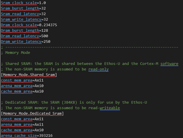
Note: The vela compilation code uses a configuration file vela.ini, which contains (amongst others) hardware-specific settings. The content of this ini file for the Alif hardware is listed at the end of this document. Vela uses the settings in this ini file to produce performance estimations, when running the model on hardware.
A vela compilation can produce an output like the following:
Network summary for model
Accelerator configuration Ethos_U55_128
System configuration Ethos_U55_High_End_Embedded
Memory mode Shared_Sram
Accelerator clock 500 MHz
Design peak SRAM bandwidth 4.00 GB/s
Design peak Off-chip Flash bandwidth 0.50 GB/s
Total SRAM used 38.52 KiB
Total Off-chip Flash used 96.53 KiB
CPU operators = 0 (0.0%)
NPU operators = 38 (100.0%)
Average SRAM bandwidth 1.06 GB/s
Input SRAM bandwidth 0.09 MB/batch
Weight SRAM bandwidth 0.15 MB/batch
Output SRAM bandwidth 0.04 MB/batch
Total SRAM bandwidth 0.28 MB/batch
Total SRAM bandwidth per input 0.28 MB/inference (batch size 1)
Average Off-chip Flash bandwidth 0.35 GB/s
Input Off-chip Flash bandwidth 0.00 MB/batch
Weight Off-chip Flash bandwidth 0.09 MB/batch
Output Off-chip Flash bandwidth 0.00 MB/batch
Total Off-chip Flash bandwidth 0.09 MB/batch
Total Off-chip Flash bandwidth per input 0.09 MB/inference (batch size 1)
Neural network macs 2822292 MACs/batch
Network Tops/s 0.02 Tops/s
NPU cycles 100225 cycles/batch
SRAM Access cycles 16940 cycles/batch
DRAM Access cycles 0 cycles/batch
On-chip Flash Access cycles 0 cycles/batch
Off-chip Flash Access cycles 35776 cycles/batch
Total cycles 132717 cycles/batch
Batch Inference time 0.27 ms, 3767.41 inferences/s (batch size 1)
Note: If the model contains operations or layers that are not supported by the Ethos-U55, then this printout will indicate that those layers are running on CPU instead.
As mentioned, the performance numbers produced by the vela compilation are the result of linear calculations using the settings in the vela.ini file. These values can deviate significantly from the performance measured on actual hardware.
The next step is to convert the model into a ‘Flatbuffer’ format that can be added to the inference code, and all together converted to binaries that can be written directly into memory.
Model Conversion into Flatbuffer Format
The ‘Flatbuffer’ is basically the model converted into an array of hexadecimal byte values. This array can then for example be included as a C header-file with the (C and/or C++) inference code used for this application.
On Linux the conversion of the model_vela.tflite file into a hex array can be done using the xxd tool. This tool can be installed on Linux with
> sudo apt install -y xxd
The conversion of the model file and inserting the hex dump into a C header-file is simply done with the following command line call:
> xxd -I output/model_vela.tflite my_network_model.h
Model File Clean-Up
Finally, the headline and footer of my_network_model.h need to be adjusted, so the linker knows how best to put the data into memory.
For this, make sure that the model file has the following framing:
#ifndef NETWORK_MODEL_H
#define NETWORK_MODEL_H
const unsigned char network_model[] __attribute__((aligned(16))) = {
…
};
const unsigned int network_model_len = nnn;
#endif //NETWORK_MODEL_H
Here “…” indicates a list of comma-separated hex byte values (e.g., 0x20). “nnn” is the size of the model array, i.e., the amount of hex byte values between the curly brackets {}.
Prepare a (Static) Inference Input
The next step is to prepare test input to run through this model for inference.
A DNN model expects input to be formatted in a specific way, which consists mostly of the following:
1. Shape the model to the same size as the data the model was trained on. For example, if images of (widthheightdepth)=(2552551) were used during the training, then the inference input needs to be shaped to this size as well.
2. Scale (or normalize) the input the same way as was done during inference. For example, if the image pixels were scaled down from 8-bit (0 to 255) to the range of 0 to 1, then also the inference input needs to be per pixels divided by 255.
3. The model we used was int-8 quantized, i.e., the inference input needs to be quantized as well using the input-scale and the zero-point values we gained during the quantization of the model.
The input data needs to be converted into a 1-D (‘flat’) array and can be in integer or in hex byte format.
The final step is to make sure that the header and footer of this input file are aligned with the rest. In this case the file can look like this:
#ifndef INPUT_DATA_H
#define INPUT_DATA_H
static const int input_data_len = 784;
static const int8_t input_data[] = {
-128, -128, -128, -128, -128, -128, -128, -128,
…
-128, -128, -128, -128, -128, -128, -128, -128
};
#endif // INPUT_DATA_H
This can be stored in a C header-file such as input_data.h, which can be linked with the C/C++ inference code.
For (Static) Inference Prepare an ‘Expected Output’ for Testing
For validation, it can be useful to compare the output of the inference from the Ethos-U55 with the “expected output”. The expected output can be generated running the test input created in “Prepare a (Static) Inference Input” after steps 1 to 3 (before the conversion into the 1-D array), using the quantized (but not yet vela compiled) model model.tflite.
It is expected that the output of the quantized model model.tflite is identical to the inference result, running the input through the vela optimized model on the Ethos-U55 hardware.
The Expected Output data is put in a header-file (e.g., called expected_output.h) and needs to be similarly formatted, as was done for the input data. This allows the expected output to be included into the inferencing binaries.
To include the expected output array into the inference code, it can be formatted as follows:
#ifndef EXPECTED_OUTPUT_DATA_H
#define EXPECTED_OUTPUT_DATA_H
static const int expected_output_data_len = 10;
static const int8_t expected_output_data[] = {
-128, -128, 127, -128, -128, -128, -128, -128,
-128, -128
};
#endif // EXPECTED_OUTPUT_DATA_H
(Note: The expected output array here is given as an example).
As the output is generated running a scaled and quantized input through a quantized model, the output is already quantized and scaled. Hence, if it is desired to get the “original” bit-depth, an additional calculation per output feature needs to be done to de-quantize and rescale the values back.
Running Inference on the MCU
With model, input and expected output as 1-D arrays, prepared as described above, we can write the C-code, for the actual inference routine. Note that this code will generally be a combination of C and C++ code, as TensorFlow lite is written mostly in C++ and needs to be included in the code.
The C-code for the inference needs to include the TensorFlow runtime libraries and other optimization functions with this header:
#include “tensorflow/lite/micro/micro_error_reporter.h”
#include “tensorflow/lite/micro/micro_interpreter.h”
#include “tensorflow/lite/micro/micro_utils.h”
#include “tensorflow/lite/micro/testing/micro_test.h”
#include “tensorflow/lite/schema/schema_generated.h”
#include “tensorflow/lite/micro/micro_mutable_op_resolver.h”
Note, the last include “micro_mutable_op_resolver.h”. During the development phase and if the working memory is large enough, this can be replaced by:
#include “tensorflow/lite/micro/all_ops_resolver.h
The “ops resolver” is what tells the NPU how to process various mathematical operations that are required to transform the input to the output (inference). “all_ops_resolver.h” contains all operations that have been implemented so far, and new ones are added to the TensorFlow repo continuously.
However, a given model requires only a limited set of operations that were used to design the model. If all operations required for the model are known, then we can instead import the “micro_mutable_op_resolver.h” file, which allows us to only pick the ops that are really required.
This can reduce the memory footprint of an application significantly.
Here is an example for a model, which is supposed to run on EthosU, contains a depth-wise convolution, a Conv-2D, an average-pooling, an add, a reshape and a softmax layer:
tflite::MicroMutableOpResolver<7> micro_op_resolver;
//tell tensorflow micro to add ethos-u operator
micro_op_resolver.AddEthosU();
micro_op_resolver.AddDepthwiseConv2D();
micro_op_resolver.AddConv2D();
micro_op_resolver.AddAveragePool2D();
micro_op_resolver.AddAdd();
micro_op_resolver.AddReshape();
micro_op_resolver.AddSoftmax();
Note that the number between the brackets <> following MicroMutableOpResolver (here 7) needs to be equal or larger than the added operator layers.
Next, we need to include model, input and expected output files with the following:
#include “my_network_model.h”
#include “input_data.h”
#include “expected_output_data.h”
An essential value, that might have to be determined experimentally, is the size of the tensor-arena:
#define TENSOR_ARENA_SIZE (70 * 1024)
The value here is given as an example. This area of memory is used to store the model’s input, output, and intermediate tensors. This value doesn’t have to be exact, so we can start with a larger value and reduce it to optimize the memory footprint.
Continuous Inference on Changing Input
The input and expected-output files (input_data.h and expected_output_data.h) are placed into memory locations specified in the linker-script. In the ARM libraries (e.g., in ml-embedded-evaluation-kit) the linker-script is called platform.ld and for the corstone-300 evaluation board can be found in dependencies/core-platform/targets/corstone-300/.
The location for the input data is specified in the linker-script with input_data_sec, the output of the inference is specified with output_data_sec and the expected output is specified there with expected_output_data_sec.
With the starting addresses and the size of each block of those memory locations specified, we can convert the single inference into an inferencing loop.
We need for continuous inference a pipeline, that continuously (or interrupt controlled) generates new input features (or frames), converts, and shapes the input as described earlier and puts the input into the specified input_data_sec. Once the input is written into the memory, the inferencing loop (ideally interrupt-controlled) picks the new input data, runs it through the NPU and places the output into the memory location of the output_data_sec.
Once the output data is written, it can be read out from the known memory address and further processed as desired, making the NPU ready for the next incoming data.
Summary
This document has given an overview of all steps required for the conversion of a quantized model into the final format required for the deployment on the Ethos-U55.
Appendix
Vela.ini